A statistical journey through the language of the Bard using Python and Zipf's Law
After learning about Zipf's Law, I embarked on a quest to find these fascinating linguistic patterns in one of the greatest bodies of work in the English language: the complete works of William Shakespeare.
This analysis was conducted as part of my Python 3 learning journey using Anaconda 4.2.0 with Python 3.5, specifically exploring file I/O, text processing, and data visualization. The complete works were sourced from The MIT Shakespeare Repository, which has been serving Shakespeare's plays and poetry to the Internet community since 1993.
Zipf's Law states that in natural language, the frequency of any word is inversely proportional to its rank in the frequency table.
In other words, the most frequent word occurs approximately twice as often as the second most frequent word,
three times as often as the third most frequent word, and so on. The mathematical formula is: f(r) ∝ 1/rα where α ≈ 1.
Total Letters Analyzed
Unique Words
Letter 'E' Count (Most Frequent)
Plays + 154 Sonnets
All 37 plays and 154 sonnets from Shakespeare's complete works were analyzed from The MIT Shakespeare Repository. The works are categorized into Comedies, Tragedies, Histories, and Poetry.
Zipf's Law is a fascinating empirical law that appears in many natural phenomena, particularly in linguistics. Named after linguist George Kingsley Zipf, it describes how word frequencies follow a predictable pattern in natural language.
f(r) ∝ 1/rα
Where f(r) is frequency, r is rank, and α ≈ 1
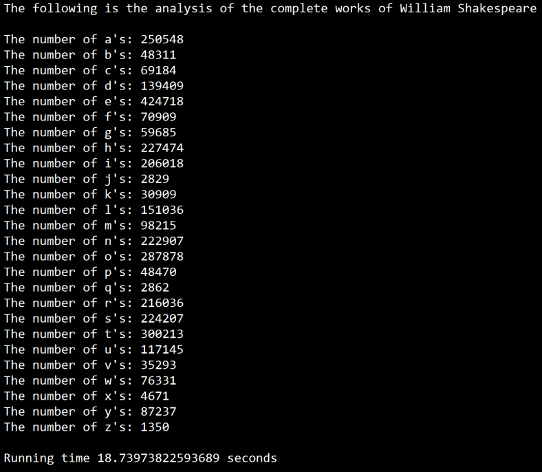
Analysis of 3,880,890 total letters across all of Shakespeare's works reveals fascinating patterns in English letter distribution. The letter 'E' dominates with over 424,000 occurrences (10.94% of all letters).
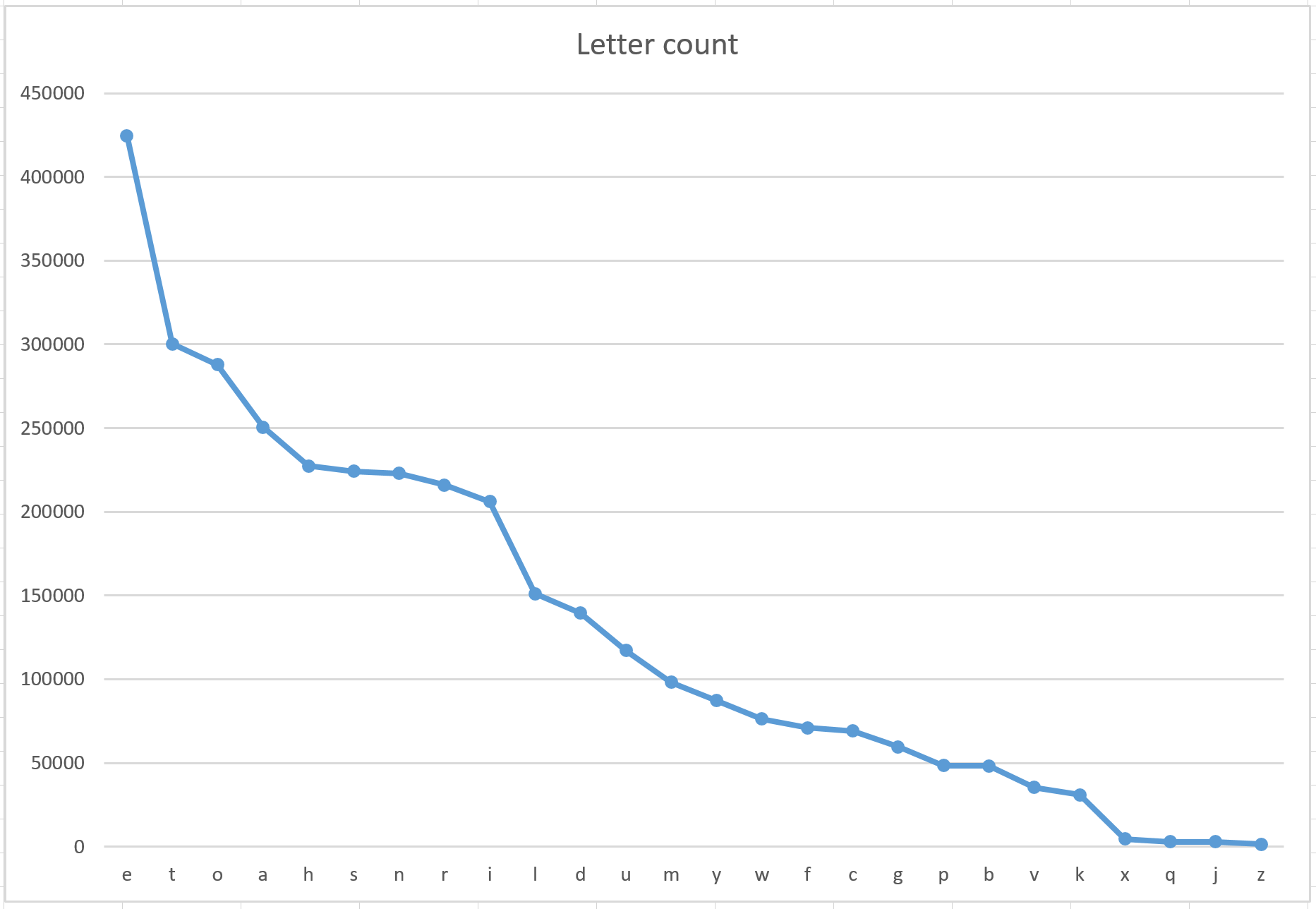
The distribution follows an exponentially decreasing pattern, characteristic of natural language letter frequency.
| Rank | Letter | Count | Percentage | Visual Distribution |
|---|---|---|---|---|
| 1 | E | 424,718 | 10.94% | |
| 2 | T | 300,213 | 7.74% | |
| 3 | O | 287,878 | 7.42% | |
| 4 | A | 250,548 | 6.46% | |
| 5 | H | 227,474 | 5.86% | |
| 6 | S | 224,207 | 5.78% | |
| 7 | N | 222,907 | 5.74% | |
| 8 | R | 216,036 | 5.57% | |
| 9 | I | 206,018 | 5.31% | |
| 10 | L | 151,036 | 3.89% | |
| 11 | D | 139,409 | 3.59% | |
| 12 | U | 117,145 | 3.02% | |
| 13 | M | 98,215 | 2.53% | |
| 14 | Y | 87,237 | 2.25% | |
| 15 | W | 76,331 | 1.97% | |
| 16 | F | 70,909 | 1.83% | |
| 17 | C | 69,184 | 1.78% | |
| 18 | G | 59,685 | 1.54% | |
| 19 | P | 48,470 | 1.25% | |
| 20 | B | 48,311 | 1.24% | |
| 21 | V | 35,293 | 0.91% | |
| 22 | K | 30,909 | 0.80% | |
| 23 | X | 4,671 | 0.12% | |
| 24 | Q | 2,862 | 0.07% | |
| 25 | J | 2,829 | 0.07% | |
| 26 | Z | 1,350 | 0.03% |
A similar analysis was performed on individual words using a Python dictionary to track unique words across all texts. The corpus contains over 30,000 unique words, with fascinating patterns emerging in the most frequently used terms.
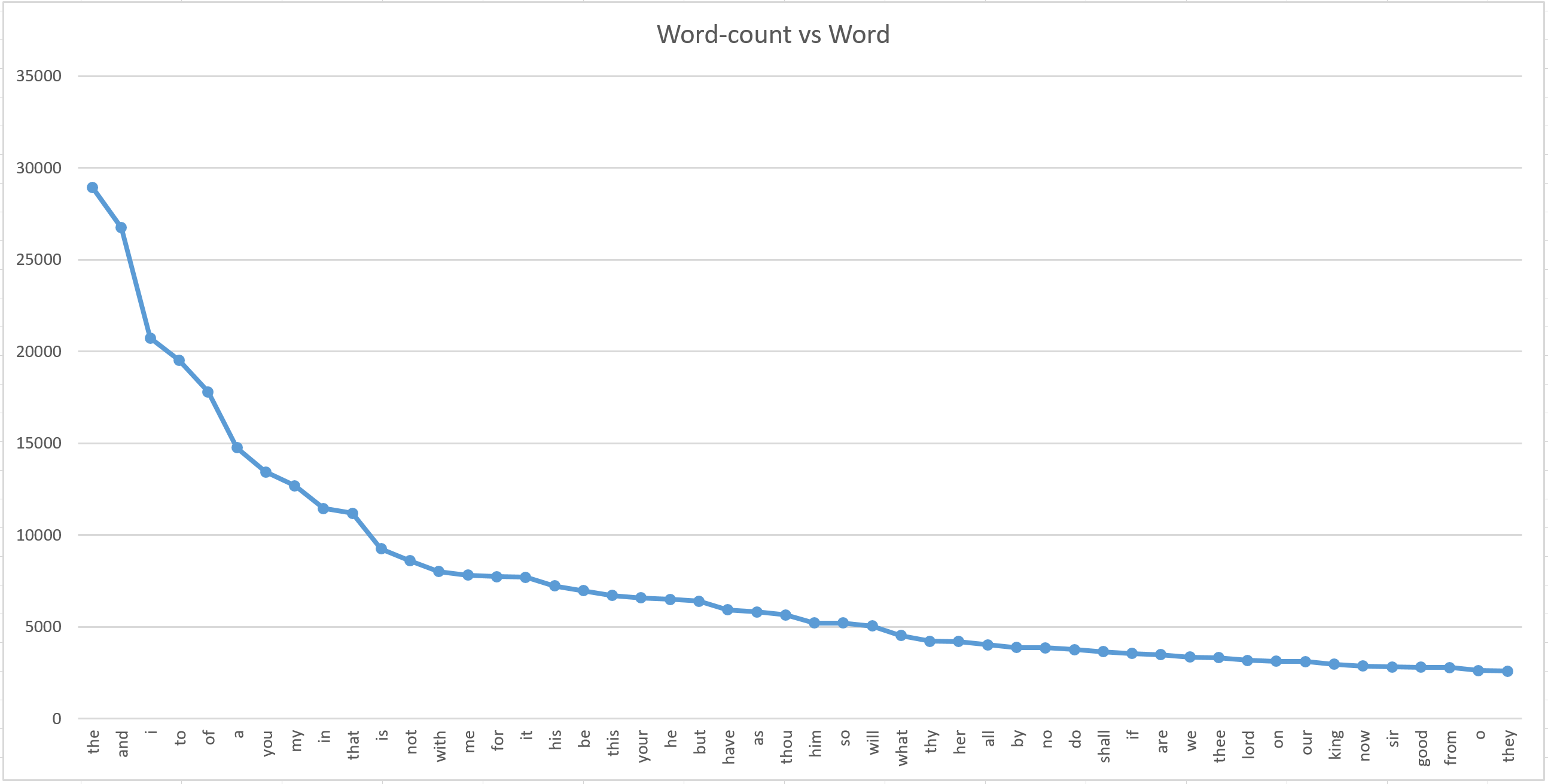
The most frequently used words include common English articles, conjunctions, and pronouns:
Shakespeare's characteristic use of Early Modern English includes frequent archaic pronouns:
Code for analyzing letter frequency distribution across all works
Code for tracking word frequency using Python dictionaries
Explore Shakespeare's works through cutting-edge D3.js visualizations. These interactive charts reveal patterns, verify linguistic laws, and provide deep insights into the Bard's language.
Bubble size represents letter frequency. Hover over bubbles for detailed statistics.
This logarithmic chart verifies Zipf's Law by plotting word rank vs. frequency. The straight line on a log-log scale confirms the inverse relationship.
Interactive donut chart showing the distribution of Shakespeare's works by genre.
Type-Token Ratio measures vocabulary diversity. Higher TTR = more varied vocabulary.
Area chart showing plays written per year. Hover over data points to see which plays were written that year.
Force-directed graph showing Shakespeare's 10 most prominent characters. Node size represents number of lines. Drag nodes to rearrange, scroll to zoom.
All visualizations are built using D3.js v7 (Data-Driven Documents), the industry-standard library for creating dynamic, interactive data visualizations.