Probability | Order Statistics | Distributions

Question

(Order Statistics) Let \(X_{(1)}, ..., X_{(n)}\) be independent and identically distributed continuous random variables with probability distribution \(F\) and density function \(F’(x) = f(x)\). If we let \(X_{(i)}\) denote the \(i_{th}\) smallest of these random variables, then \(X_{(1)}, ..., X_{(n)}\) are called the order statistics. To obtain the distribution of X(i), note that X(i) will be less than or equal to x if and only if at least i of the n random variables \(X_{(1)}, ..., X_{(n)}\) are less than or equal to \(x\).

Solution

Putting this problem in another way, let us say you generate a list of random numbers. For the example’s sake let the variate be having a standard normal distribution. Here is a list of 10 random normal numbers. \[\{-1.04703, -0.273997, 0.850384, 0.277371, 1.39499, 1.03797, -0.266823, 0.501695, 0.929459, 0.971281\}\] Now we order the list, \[\{-1.04703, -0.273997, -0.266823, 0.277371, 0.501695, 0.850384, 0.929459, 0.971281, 1.03797, 1.39499\}\]

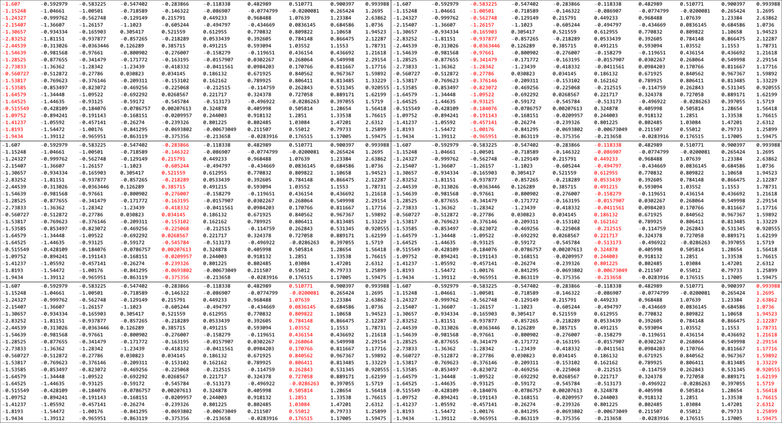
If we have several of these ordered lists, we are interested in what the density of the distribution of an \(i^{th}\) element from across several lists (or samples) would be. The image below shows the one such list of numbers. Observe that each row is ordered and we take the “similarly ranked” elements and look at their distributions. In the image, we would be taking each column at a time and looking at their distributions. For fitting the table in a single page, I have only taken 10 number per row. In this next section we would see the distributions for different sample sizes.

Unsorted table looks like this

sorted table looks like this

The image below is an animation. It might take a few seconds to load.

Standard Normal Distribution


Module[{data, divisions = 30, plots, chartTypes = {"PointDensity", "HistogramDensity", "SmoothDensity"}},
    data = Transpose[Sort[#] & /@ RandomVariate[NormalDistribution[], {1000, divisions}]];
    plots = DistributionChart[Join @@ {{Flatten@data}, data}
        , ChartLabels -> Join @@ {{Style["All", Red]}, Style[Subscript["x", ToString[#]], 12] & /@ Range@divisions}
        , ImageSize -> 788
        , AspectRatio -> 0.5
        , GridLines -> {Range[divisions + 1], Range[-6, 6, 1]}
        , ChartElementFunction -> #
        , AxesLabel -> {"Distribution", "Rank of the random number"}] & /@ chartTypes;
    Export[StringReplace[NotebookFileName[], ".nb" -> "_normal_" <> ToString[chartTypes[[#]]] <> ".svg"], plots[[#]]
    , ImageSize -> 788
    , ImageResolution -> 500] & /@ Range@Length@chartTypes
 ]

The data consists of 1000 vectors each with a length of 30. After the individual vectors have been sorted, the random numbers of ranks 1 through 30 have been extracted and the distributions of these ranked random numbers have have been shown sequentially.
Plot: The first distribution in each of the chart shows the complete data, the smaller ranged variables that are following these are the ranked numbers. For example, x1 is the distribution of the all the smallest numbers in each of the vector. This that x1 is made of 1000 numbers.
Observe how the range of the rank is heavily dependent on the rank of the variable itself within its own sample (or vector here)

Note: All the three images below are showing the same data with a different “ChartElementFunction”

Standard Uniform Distribution


Module[{data, divisions = 30, plots, chartTypes = {"PointDensity", "HistogramDensity", "SmoothDensity"}},
    data = Transpose[Sort[#] & /@ RandomVariate[UniformDistribution[], {1000, divisions}]]
    plots = DistributionChart[Join @@ {{Flatten@data}, data}
        , ChartLabels -> Join @@ {{Style["All", Red]}, Style[Subscript["x", ToString[#]], 12] & /@ Range@divisions}
        , ImageSize -> 788
        , AspectRatio -> 0.5
        , GridLines -> {Range[divisions + 1], Range[-6, 6, 1]}
        , ChartElementFunction -> #
        , AxesLabel -> {"Distribution", "Rank of the random number"}] & /@ chartTypes;
    Export[StringReplace[NotebookFileName[], ".nb" -> "_normal_" <> ToString[chartTypes[[#]]] <> ".svg"], plots[[#]]
    , ImageSize -> 788
    , ImageResolution -> 500] & /@ Range@Length@chartTypes
 ]

The data creation method is the same as explained above for the normal distribution.

Exponential Distribution with \(\lambda=1\)


Module[{data, divisions = 30, plots, chartTypes = {"PointDensity", "HistogramDensity", "SmoothDensity"}},
    data = Transpose[Sort[#] & /@ RandomVariate[ExponentialDistribution[1], {1000, divisions}]];
    plots = DistributionChart[Join @@ {{Flatten@data}, data}
        , ChartLabels -> Join @@ {{Style["All", Red]}, Style[Subscript["x", ToString[#]], 12] & /@ Range@divisions}
        , ImageSize -> 788
        , AspectRatio -> 0.5
        , GridLines -> {Range[divisions + 1], Range[-6, 6, 1]}
        , ChartElementFunction -> #
        , AxesLabel -> {"Distribution", "Rank of the random number"}] & /@ chartTypes;
    Export[StringReplace[NotebookFileName[], ".nb" -> "_normal_" <> ToString[chartTypes[[#]]] <> ".svg"], plots[[#]]
    , ImageSize -> 788
    , ImageResolution -> 500] & /@ Range@Length@chartTypes
 ]

Chi-Square Distribution with \(k=1\)


Module[{data, divisions = 30, plots, chartTypes = {"PointDensity", "HistogramDensity", "SmoothDensity"}},
    data = Transpose[Sort[#] & /@ RandomVariate[ChiSquareDistribution[1], {1000, divisions}]];
    plots = DistributionChart[Join @@ {{Flatten@data}, data}
        , ChartLabels -> Join @@ {{Style["All", Red]}, Style[Subscript["x", ToString[#]], 12] & /@ Range@divisions}
        , ImageSize -> 788
        , AspectRatio -> 0.5
        , GridLines -> {Range[divisions + 1], Range[-6, 6, 1]}
        , ChartElementFunction -> #
        , AxesLabel -> {"Distribution", "Rank of the random number"}] & /@ chartTypes;
    Export[StringReplace[NotebookFileName[], ".nb" -> "_normal_" <> ToString[chartTypes[[#]]] <> ".svg"], plots[[#]]
    , ImageSize -> 788
    , ImageResolution -> 500] & /@ Range@Length@chartTypes
 ]

Gamma Distribution with \(k=2, \theta=2\)


Module[{data, divisions = 30, plots, chartTypes = {"PointDensity", "HistogramDensity", "SmoothDensity"}},
    data = Transpose[Sort[#] & /@ RandomVariate[GammaDistribution[2, 2], {1000, divisions}]];
    plots = DistributionChart[Join @@ {{Flatten@data}, data}
        , ChartLabels -> Join @@ {{Style["All", Red]}, Style[Subscript["x", ToString[#]], 12] & /@ Range@divisions}
        , ImageSize -> 788
        , AspectRatio -> 0.5
        , GridLines -> {Range[divisions + 1], Range[-6, 6, 1]}
        , ChartElementFunction -> #
        , AxesLabel -> {"Distribution", "Rank of the random number"}] & /@ chartTypes;
    Export[StringReplace[NotebookFileName[], ".nb" -> "_normal_" <> ToString[chartTypes[[#]]] <> ".svg"], plots[[#]]
    , ImageSize -> 788
    , ImageResolution -> 500] & /@ Range@Length@chartTypes
 ]